Popular information
English
Swedish

Information for the Public
Statistical Methods for Economic Time Series
When estimating relationships, making forecasts and testing hypotheses from economic theory, researchers frequently use data in the form of time series – chronological sequences of observations – to study macroeconomic variables. Consumption in an economy may thus depend on total labor income and wealth, real interest rates, the age distribution of the population, etc. The simplest conceivable textbook example of such a relationship is a static, linear expression with only two variables:

According to this equation, the variable gt (for instance, consumption in quarter t) depends on the variable xt (for instance, income during the same period). The last, random-error, term et denotes the variation in gt which cannot be explained by the model. By means of time series for the variables gt and xt, the parameters a and b can be estimated using statistical methods (known as regression analysis). Valid conclusions presuppose that the methods are well adapted to the specific properties of the time series. This year’s laureates have developed methods that capture two key properties of many economic time series: nonstationarity and time-varying volatility.
Nonstationarity, Common Trends and Cointegration
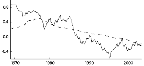
Many macroeconomic time series are nonstationary: a variable, such as GDP, thus follows a long-run trend, where temporary disturbances affect its long-term level. In contrast to stationary time series, nonstationary series do not exhibit any clear-cut tendency to return to a constant value or a given trend. Figure 1 shows two examples of such time series. The jagged curve, with large short-run variations, represents the exchange rate between the Japanese yen and the U.S. dollar for each month since 1970. The smoother curve shows the consumer price level in Japan in relation to that in the U.S. during the same period.
 |
| High resolution image (jpeg 110 kB) |
| Figure 1: Logarithm of the Japanese yen/U.S. dollar exchange-rate index and the logarithm of the quotient between the consumer price index for Japan and the consumer price index for the U.S.; monthly observations, January 1970–May 2003. |
Statistical Pitfalls
For a long time, despite the fact that macroeconomic time series are often nonstationary, researchers only had access to standard methods developed for stationary data. In 1974, Clive Granger (and his colleague Paul Newbold) demonstrated that estimates of relationships between nonstationary variables could yield nonsensical results by erroneously indicating significant relationships between wholly unrelated variables. (In the above equation, the problem arises if the random error et is nonstationary. A standard test may then indicate that b is different from 0, even though the true value is 0.)
Statistical pitfalls can also give rise to misleading results in cases where a relationship does in fact exist. In particular, it may be difficult to distinguish between temporary and permanent relationships among nonstationary time series. For example, economic theory postulates that, in the long run, a stronger exchange rate should be associated with relatively slower price increases, because prices expressed in a common currency cannot deviate too much from one another. Such a tendency is also revealed in Figure 1, where the yen became stronger against the dollar over the period, while the price level in the U.S. rose in relation to the Japanese price level. In the short run, however, expectations and capital movements have such a pervasive effect on the exchange rate that standard methods may be inadequate for precise estimation of the long-run relationship.
A common approach to dealing with the problem of nonstationary data had been to specify statistical models as relationships between differences, i.e., rates of increase. Instead of using the exchange rate and the relative price level, one would estimate the relationship between currency depreciation and relative inflation. If the rates of increase are indeed stationary, traditional methods provide valid results. But even if a statistical model based solely on difference terms can capture the short-run dynamics in a process, it has less to say about the long-run covariation of the variables. This is unfortunate because economic theory is often formulated in terms of levels and not differences.
Owing to the properties of nonstationary data, it therefore became a challenge to find methods which could trace the potential long-run relationships concealed by the noise of short-run fluctuations. The work of Clive Granger has generated such a methodology for statistical analysis.
Granger’s Contribution
In research published during the 1980s, Granger developed concepts and analytical methods that combine short-run and long-run perspectives. The key to these methods, and to valid statistical inference, is his discovery that a specific combination of two (or more) nonstationary series may be stationary. Economic theory often makes exactly such predictions: if there is an equilibrium relationship between two economic variables, they may deviate from the equilibrium in the short run, but will adjust towards the equilibrium in the longer run. For example, conventional theory predicts a long-term equilibrium exchange rate, where price levels expressed in a common currency are on parity with each other. Granger minted the term cointegration for a stationary combination of nonstationary variables.
Granger also demonstrated that the joint dynamics among cointegrated variables may be expressed in a so-called error-correction model. Such a model is not only statistically sound, but can also be given a meaningful economic interpretation. For example, the dynamics in exchange rates and prices are driven by two simultaneous forces: a tendency to smooth out deviations from the long-run equilibrium exchange rate, and short-run fluctuations around the adjustment path towards this long-run equilibrium.
The concept of cointegration would not have become useful in practice without powerful statistical methods for estimation and testing of hypotheses. Clive Granger and Robert Engle introduced such methods in a remarkably influential article published in 1987. Here, they present a test of the hypothesis that a number of nonstationary variables are not cointegrated, as well as a two-step method for estimating the error-correction model. Improved methods, which have now become standard, were later developed by Søren Johansen.
In subsequent work and in collaboration with other researchers, Granger has extended cointegration analysis in several respects, including the ability to handle series with seasonal patterns (seasonal cointegration) and series where adjustment towards equilibrium does not occur until the deviation exceeds a critical value (threshold cointegration).
Applications
Clive Granger’s work has transformed the way economists deal with time-series data. Today, tests of stationarity and cointegration are carried out routinely as a stepping-stone to the specification of dynamic econometric models. Cointegration analysis has turned out to be particularly valuable in systems where short-term dynamics are affected by large random disturbances, while long-term variations are simultaneously constrained by economic equilibrium relationships. An example is the relation between exchange rates and price levels. Other examples include the relation between consumption and wealth (which have to be consistent with one another in the long run, although consumption is much smoother than wealth in the short run), dividends and stock prices (where stock prices follow the development of dividends in the long run, but exhibit substantially larger fluctuations in the short run) and interest rates of different maturities (where long and short rates are linked together by expectations regarding future short rates, even if they move in different directions in the short run).
Time-Varying Volatility and Arch
Risk evaluation is at the core of activities on financial markets. Investors assess expected returns of an asset against its risk. Banks and other financial institutions would like to ensure that the value of their assets does not fall below some minimum level that would expose the bank to insolvency. Such evaluations cannot be made without measuring the volatility of asset returns. Robert Engle developed improved methods for carrying out these kinds of evaluations.
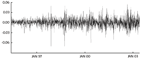
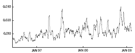
Figure 2 shows the returns on an investment in the NYSE stock index (the Standard & Poor 500) for all stock-market days between May 1995 and April 2003. The returns averaged 5.3 percent per year. At the same time there were days, when the fluctuations in prices were greater (plus or minus) than 5 percent. The standard deviation* in daily returns measured over the entire period was 1.2 percent. Closer inspection reveals, however, that the volatility varies over time: large changes (upwards or downwards) are often followed by further large fluctuations, and small changes tend to be followed by small fluctuations. This is clearly illustrated in Figure 3, which shows how the standard deviation, measured over the last four weeks, moved over time. Evidently, the standard deviation varied considerably, from approximately 0.5 percent during calm periods to nearly 3 percent during more turbulent episodes. Many financial time series are characterized by similar time variation in volatility.

High resolution image (jpeg 287 kB)
Figure 2: Percentage daily returns on an investment in the Standard & Poor 500 stock index, May 16, 1995–April 29, 2003.
 |
| High resolution image (jpeg 161 kB) |
| Figure 3: Standard deviation for percentage daily returns on an investment in the Standard & Poor 500 stock index, May 16, 1995–April 29, 2003, computed from data for the four preceding weeks. |
Engle’s Contribution
Figure 3 shows backward-looking calculations of time-varying volatility. But investors and financial institutions need forward-looking evaluations – forecasts – of volatility during the next day, week and year. In an outstanding article in 1982, Robert Engle formulated a model which allows such evaluations.
Statistical models of asset returns can only explain a fraction of the variation from one day to the next. Most of the volatility is thus embedded in the random error term (et in the introductory equation) – or, in other words, in the model’s forecasting error. In standard statistical models, the expected variance of the random error is assumed to be constant over time. Obviously, this is far from capturing the large variations in asset returns depicted in Figure 3.
Engle assumed instead that the variance of the random error in a certain statistical model, in a certain time period, systematically depends on previously realized random errors, so that large (small) errors tend to be followed by large (small) errors. In technical terms, the random variable displays autoregressive conditional heteroskedasticity. His approach has therefore become acronymized ARCH. In our example, the model now contains not only a forecasting equation for asset returns, but also a number of parameters showing how the variance of the random error in this equation depends on forecasting errors in earlier periods. Engle demonstrated how ARCH models could be estimated and introduced a practical test for the hypothesis that the conditional variance of the random error is constant.
In subsequent work and in collaboration with students and colleagues, Engle developed this concept in several different directions. The best-known extension is the generalized ARCH model (GARCH) developed by Tim Bollerslev in 1986. Here, the variance of the random error in a certain period depends not only on previous errors, but also on the variance itself in earlier periods. This development has turned out to be very useful; GARCH is the model most often applied today.
Applications
In his first article on ARCH, Engle used his model of time-varying volatility to study inflation. Not before long, however, it became clear that the most important applications were to be found in the financial sector, where activities aim at handling and pricing different types of risk. Price-setting models thus represent the relation between prices of securities and volatility: the expected returns on specific shares depend on the covariance between the return on the share and the market portfolio (according to the CAPM developed by Sharpe, Economics Laureate in 1990), option prices depend on the variance in the return on the underlying asset (according to the Black-Scholes formula, awarded the Economics Prize in 1997 to Merton and Scholes), etc.
In joint work with other researchers, Engle has captured these relationships by developing models (GARCH-M) where expected returns depend on time-varying variances and covariances, thereby becoming time-varying themselves.
What are the practical implications of time-varying volatility? If a GARCH model is applied to the stock returns in Figure 2, conditional volatility, expressed as a standard deviation, fluctuates between 0.5 and 3 percent during the period in question. If an investor has a portfolio corresponding to the Standard & Poor 500, how much capital would she risk losing the next day? Given a forecasted standard deviation of 0.5 percent, her loss – with 99 percent probability – would not exceed 1.2 percent of the value of the portfolio. If the forecasted standard deviation were 3 percent, the corresponding capital loss would be as high as 6.7 percent. Similar calculations of value at risk are crucial in modern risk analysis when banks and other institutions compute the market risk in their securities portfolios. Since 1996, an international agreement (the so-called Basle rules) also prescribes the use of value at risk in the control of banks’ capital requirements. Through its use in these and other contexts, the ARCH frame-work is an indispensable tool for risk assessment in the financial sector.
* The standard deviation is defined as the square root of the variance, which gives the average squared deviation from the mean value of a series. The variance for T observations of a variable xt with mean value ![]() can thus be computed as
can thus be computed as ![]()
The Laureates
Robert F. Engle
New York University
Salomon Center
44 West Fourth Street, Suite 9-62
New York, NY 10012-1126
USA
American citizen. Born in 1942, in Syracuse, NY, USA. Ph.D. from Cornell University in 1969; Michael Armellino Professor of Management of Financial Services at New York University, NY, USA.
Clive W. J. Granger
Department of Economics
University of California, San Diego
9500 Gilman Drive
La Jolla, CA 92093-0508
USA
British citizen. Born 1934, in Swansea, Wales. Ph.D. from University of Nottingham in 1959; emeritus Professor of Economics at University of California at San Diego, USA.
